The Jedox Roadshow comes to Brisbane

Jedox is one of the best unknown data platforms I know of.  Calling them unknown may sound a little harsh because they are a major product however, I say unknown because I don’t see them being considered for purchase in a large number of companies when they are clearly a fit for purpose product – and the best one at that.

For budgeting applications and situations where users need 2 way interaction with data – they ROCK.  Consider a budgeting example where you say something like ‘apportion $5000 like last year’, or ‘apportion $5000 evenly’ , jeodx just takes care of it.  And if you want comment why you decided to make that allocation, you can.  For financial budgeting, there is just no better product.  There’s automatic Excel integration, report authoring from Excel with publish to the Web, so accountants, planners , analysts and alike find it easy and natural to use.

I’m always keen when things are on in Brisbane and they’ll be here on 19th May (2017).  You can find out more here.

Schema Definitions from an ODBC Text Source

Recently, I’ve worked on disjointed migration project where things just didn’t work the way you expect.  For example, you usually like to access data direct from its source (direct from a relational database) but in this situation, this was just not allowed and we were given a load of text files (hundreds) to load.  Perhaps not so bad, you may say however, unfortunately, the documentation around those files was incomplete and incorrect.  It seems that we spent for too much time confirming valid formats and playing too and fro with vendors – Its not really value adding and lets face it, its not really a good use of time to transfer and manually configure text import.  So what could we do?  All files were deposited in a directory, so why not use the Schema collections from an ODBC source?

The idea is to setup an ODBC source that points to the directory with files in it, create a connection to that source and then use the meta data of that connection to iterate over each table in the source and get the column information from that table.  Note that for a text driver, each file represents a table and that’s why I refer to tables above.

1. Setting Up the Driver

I think this is relatively straight forward so I’ll just add the key points with a word of warning.  There is no x64 bit driver installed by default for windows, so you may want to download the Access one from here if you need to.  Access the ODBC drivers from your settings (just type ODBC in the search bar and then choose to setup a connection or access ODBC sources), then just add a new source and choose the text driver.

When you click Finish you’ll be presented with the window below where you can specify the directory you want to use and give the source a name (see below).  There’s no need to look at options, but if you want to, you can specify specific extensions but for now lets assume that everything in the folder is for import.

2. Data Access

As a side note, after you’ve set up the driver, you can now import the data as a table into Excel.  The menu path is (Data Tab) Get External Data > From Other Sources > Microsoft Query.  I know you could import the file directly (ie Get External Data > From Text) however, you want to use the text driver and text your ODBC source.  You’ll notice that this source is available as a database (see below), and each file in the directory is presented as a table.  The source that I previously created is shown below and you can see the following list of tables.

 

3. Using the ODBC Shema Object

As a general rule, when we create a database connection in code, the connection object is accompanied by a schema and we can use this to interrogate  the source.  As you can see from the snippet, all we do is acquire the “tables” schema (ie list the tables), then iterate over each table to get the columns in that table.  The sample output this shown below and, as you can see, it defines the column names and types.

            OdbcConnection _con = new OdbcConnection("DSN=biml_text_files");
_con.Open();

DataTable _schema = _con.GetSchema();
DataTable _restrictions = _con.GetSchema("Restrictions");
DataTable _tables = _con.GetSchema("Tables");

foreach (DataRow _tablerow in _tables.Rows)
{
Console.WriteLine("{0}", _tablerow["TABLE_NAME"]);

string[] _table_restrictions = { null, null, _tablerow["TABLE_NAME"].ToString() };
DataTable _columns = _con.GetSchema("Columns", _table_restrictions);
foreach (DataRow _colrow in _columns.Rows)
{
Console.WriteLine("\t{0},{1},{2}", _colrow["COLUMN_NAME"], _colrow["TYPE_NAME"], _colrow["COLUMN_SIZE"]);

}

}


_con.Close();

Actually, you don’t even need to go to this trouble.  You could just get the columns schema without the restrictions which will give you a complete list of all columns for every table.  However, in our implementation, the data was sent back to a database so others could use it.

Conclusion

Working with the Schema Information objects allows us derive information about the source.  Its conceptually similar to the INFORMATION_SCHEMA tables in most databases however, when we apply this to text files, we can use that meta-data to build our ETL.

BI Success – Does the tail wag the dog?

I am watching recorded event this morning about the keys to Business Intelligence success. The top 4 points that were provided are;

1. Finding the right (executive sponsor)
2. Don’t build what they ask for, build what they need
3. Offer up a buffet (deliver multiple options)
4. Don’t try to boil the ocean.

Lets be honest, there’s nothing new here – having the right sponsor has been listed as a critical success factor numerous times. So, to paraphrase, the presentation was basically talking about finding the correct person and delivering something that truly works for the business in an incremental approach. Why incremental? Well, I guess, (if I have my skeptics hat on) I’d suggest its better to fail fast with small outcomes so the risk adverse manager doesn’t get tagged with a failed project. On the positive note, it better aligns the business outcomes with whats delivered, reduces inertia to adoption and maintains focus on outcomes (from both the business and those delivering).

What raised my eyebrows was the first choice, finding the right sponsor. This is so important that, without doubt, I’d suggest that any rouge project would eventually be killed if it doesn’t have the right ‘executive’ support (if you don’t think so tell me otherwise). I’ve delivered remarkable shadow IT projects that were canned and aggressively removed by IT departments. For example, I’ve had the business users refuse to use the corporate system and ask IT to build systems that work like the existing one (that was built by my team).

Before you suggest that there is some valid reason why this needs to happen let me assure you there’s not. Some common arguments include statements like its not valid because it lacks IT structure, backups, testing, validation and so on. They did so there’s no technical reason why the tool’s have been killed. So I reflect on the first point that was raised in the webinar – executive sponsorship.

Now to the main point of this post, why is executive sponsorship so important? Some common arguments are that it ensures appropriate resources and organizational focus however, I cant help wondering if these are recursive justifications – somewhat aligned to the chicken and the egg, its hard to truly figure out which comes first. Is there some strategic and leadership focus here or does it reflect more about the structure of organizations?

Could the requirement for executive support be an indication of organizational compliance rather than effective management? For example, if executive John Bloggs is behind the project no one dares speak up against its short comings and so it can’t be a failure.  So, we’ll change the definition of success (scope or cost) because it appeases John Bloggs expectations and influence.

I know that there are cases where focused executives have played an active role in delivery and provided a positive impact to projects but I cant help feeling that, sometimes, the tail is wagging the dog.

Now for the ultra positive and the additional factor which I cant help thinking what comes first.  I’ve been lucky enough to work in a variety of organizations and have seen a lot of different management styles.  However, from the organizational point of view, does it not say something about the organization (and the type of people who work there) when executives actively back the project?  I am sure that something people feel passionate about and work towards will be successful, so is it not the organization rather that the politics that drives success?  That is, if executives are willing to get support the project (rather than treat it like a political football), because that’s the type of people they are, then how can it not be a success?

What are your experiences?

Data Vault (CDVDM) Training Down Under

If your looking to get some great Data Vault training in Australia in March, the Genesee academy is running the CDVDM course in Brisbane, Melbourne and Sydney.  You can get the schedule dates at the Genesee site.  It’s a great course and well worth the investment for anyone looking to get in to Data Vault data warehousing.

Automation of Excel Macros

There is still a huge value of reporting and using Excel for end users.  Excel is simple to work with, allows data access and allows end users to program with minimal learning.  As users develop their skills they inevitably look at automation through macros.  So if we want to turn this into something a little more ‘supported’ (by the corporate IT department) so that its scheduled on some manner, we’ll have to turn to a bit of programming.  So, lets look at how we can do this.  Firstly we’ll look at some rudimentary code and then we’ll look at scheduling.

Code

So here is a snippet to do that (including the reference).  You’ll notice that there are a couple of key features.  There are 2 parameters passed (the file name and the macro), then (in code) we simply open excel, then the workbook, execute the macro and save and close the workbook (and application)

using xls = Microsoft.Office.Interop.Excel;

static void Main(string[] args)
 {

    xls.Application _x = null;
     xls.Workbook _wb = null;

    string _filename = args[0];
     string _macro = args[1];

    _x = new xls.Application();
     _x.Visible = false;
     _wb = _x.Workbooks.Open(_filename);
     _x.Run(_macro);
     _wb.Save();
     _wb.Close();
     _wb = null;
     _x.Quit();
     _x = null;

}

So, if I want to run my code from the command console, you’d just run the following (note the macro is called main).

ExcelManager.exe “this-is-the-excel-workbook-name” “main”

or as a SQL Command, wrap it in a batch and then execute;

EXEC master..xp_CMDShell ‘c:\temp\excel_manager.bat’

A Gotcha

In debug mode, this all worked and the task could be scheduled and executed in windows scheduler.  However, when the the tasked was scheduled (SQL Server agent) or scheduled to run when a user was not logged in there would be be errors.  This related to file not found errors and other (generally other unhelpful and unreliable messages).  It turns out, that you’ll need to ensure that there are some folders required (don’t ask me why).  You may want to check if the following folders exist.  If not, try adding them;

C:\Windows\System32\config\systemprofile\Desktop
C:\Windows\SysWOW64\config\systemprofile\Desktop

An example of one of the type of errors you may get is;

Great Courses Down Under

For all Australian readers, there are a couple of great courses coming to Australia. 

Firstly, Barry Devlin is running a 2 day course from 24th August (see here).  For those that don’t know Barry, he is the un-official farther of data warehousing.  There at the start and  never go the media attention of others.  What I like about his approach (and specifically his later work) is that he challenges the status quo of data warehousing and information management.

Secondly, Hans Hultgren is running Data Vault certifications in July. You can find our more here AND, there is also a course being run in Brisbane (at our offices). If you want to get into Data Vault, I think this is a really great place to start.

If you want to find out any information about either of these courses, please feel free to ping me direct.

Chernoff Faces, R and Power BI

One of my favorite visualizations are Chernoff faces because they allow you to incorporate many attributes into a single visualization.  Compared to a bar chart (which only displays one attribute), you can get a ‘full picture’ of the situation in a single iconic image (pardon the pun).  Further, faces are a natural recognizable characteristic (for us humans) and this a fair bit of evidence to suggest you notice things in faces a lot easier than bland representations as a result of our social upbringing.  This post is about implementing Chernoff faces in Power BI (through R).  Firstly (in this post), I will the infamous crime statistics demonstration, and in the second post, I’ll show child faces against different dataset (Northwind) which incorporates normalization.

If you are not familiar with Chernoff faces, you can read more about them at Wikipedia here but basically they use facial characteristics to display an attribute value.  For example, the size (height) of the face may be related to income, the width of the face might be related to quantity with the size of the eyes related to margin.

Chernoff implementation in R

I will include only a snippet of R required to show Chernoff faces (and then the output).  A more complete tutorial can be found here and here.  Basically, we need to install the library, get some data and then display the visual.  This can be done with the following snippet;

install.packages(“aplpack”) # install the package
library(‘aplpack’)
crime <- read.csv(“http://datasets.flowingdata.com/crimeRatesByState-formatted.csv”) #get the data
faces(
  crime[,2:8]
  ,face.type=0
  ,scale=TRUE
  ,main=’Crime Stats USA’
  ,labels=crime$state
  ,print.info=TRUE
)  #plot the chart

We then get the face visual (as below)

Chernoff implementation Power BI

In Power BI, there are a few things we need to do.  These are;

1. Setup Power BI for R
2. Get our data (or build our model)
3. Add the visualization (by)
   1. Telling the R (custom component R visualization what data to use) and
   2. Use R code to create/format the visualization

These steps are followed below;

1. Setting up Power BI for R

Before you can use R in Power BI, you need to install that are is installed on your local machine and that you have set and enabled R’s working directories in Power BI.  To set R options in Power BI use the File > Options and settings > Options menu path.  You can see that the directory of R needs to be set and you need to allow R to plot a visual in Power BI (this is a preview feature).  I’ve included these images show the both the R directory setting and the use of R to plot visuals.

Once these features are enabled, you should see the R icon appear in your Visualisations pane (note that you’ll need to restart Power BI if you enabled R as in the above checkbox).

2. Get Data

Usually we expect to have a data model in Power BI (that is, we have imported some data, built a model and now we want to visualize it).  For this demo though, I want to import the same data set that I used in the above snippet so I can use the R Script data source in Power BI.  Here, all I have to do is choose the R source (accepting that this is a preview connector), and paste the R (read) script into the R dialog that Power BI Shows.  This is shown in the 2 images below;

After this occurs, Power BI opens up the Data Navigator and you can either Load or Edit the Import query.  I’ll just Load it (as shown below)

3. Add the Visualization

Once we have data in our Power BI workbook (you’ll notice that we have a crime table), all we need to do is;

1. add the R visualization to the page canvas
2. enable the script component (after all its custom component)
3. add the data (that the visualization uses) and
4. code the visualization (in R).  Note that the data available in R code (ie the data frame) is defined by the data that was added in the prior step. 

I have tried to show all these steps in the image below.  One thing to note about adding data to the visualization is that the order in which you add fields (from the model) defines the columns that are in the data frame.  This is important (for the Chernoff faces in R) because the first fields of the data frame defines the axis (grouping) of faces.  Note that you can also see this order in R script editor in Power BI (the code is in the image below and un-editable in Power BI but looks like # dataset <- data.frame (  columns )).

 

You may recall (from the R script above) that we referred to crime as a data frame in R when we built created the code in R.  In Power BI however, the data frame is referred to as dataset so in order to use our original code, we need to either create a new data frame in R (called crime) or change our existing R code to use a data frame called dataset.  I’ll go with the first option and paste the following code into the R script editor (where you see ‘Paste or type your R-script code here).

crime <- dataset
library(‘aplpack’)
faces(
  dataset[,2:8]
  ,face.type=0
  ,scale=TRUE
  ,main=’Crime Stats USA’
  ,labels=crime$state
  ,print.info=TRUE
)  #plot the chart

In order to change the visual (while still editing code), just press the run button (in the R Script editor).  My Power BI screen now looks like the following;

Of course the great thing about Power BI is that there is automatic filtering among visuals on the page.  The next thing to do is add a slicer for state and allow the user to select what states to show.  The R visual updates automatically.  Doing this we can easily build a visual that allows the user to select and compare the faces of the states they select (as below).

Getting Started with Biml Video

I am a huge fan of Biml and think that the ability to conceptually model data movement produces huge benefits when compared to the more traditional methods.

It must also strike a chord with others because my first post on biml has been made into a video by the folks at webucator.  You can check it out below or try the YouTube link.

Temporal Tables != Data Warehouse

With the release of SQL2016 just around the corner, there are an increasing number of posts appearing about new features that mean I don’t have to work.  One post (which motivated me to write this) claimed that this breakthrough would mean we no longer needed to store historical values – an interesting interpretation of a Data Warehouse to say the least.  Microsofts own content (here) recommends that there are huge productivity benefits in Slowly Changing Dimensions because you can compare the same key at two points in time.

The idea’s of temporary tables (recording every change to a table in an table_History table) is a cool feature – don’t get me wrong, I think its great.  However, there is (sadly) a lacking
amount of discussion about how the feature can be incorporated into the Data Warehouse.  Those that blindly follow the sales pitch “I don’t need a data warehouse” because I’ve got history tracking or perhaps “yeah, I’ve got a data warehouse – its a history tracked OLTP” will ensure their users cant get the data they need.

So lets call out some issues with reliance on temporal tables as a data warehouse replacement (and bring some data warehouse assumptions to the surface).  I will focus on the star schema design since most references explicit refer to changing dimensions (however we can apply these ideas to other methodologies).

A fundamental construct of the star schema is the surrogate key (almost as fundamental as the concept of dimension and fact).  Using the surrogate uniquely identifies an instance of a dimension at a point in time and therefore, state of the dimension can be precisely identified for the fact record.  For example, if I sold a product on a date, I need to look up the product dimension and determine which version of the product was applicable on that date.  The products surrogate key (not the Product Id or Code) is used in the fact.  This is the fundamental design of the star schema.  A temporal table does not provide you the capacity to do this – all it can do is provide the data to construct the star. 

How could you solve this with temporary tables?  Well, there may be the thought that you could concatenate the tables primary key and the records start date for uniqueness and then determine what (dimension) record is applicable to a fact record via a query.  Interesting idea but not something I’d take on litely.  I suspect that performance would degenerate so quickly both the BI users and the Ops users (remember that this is occurring on the OLTP) would walk away in droves.  Remember that this has to occur for every record in the fact – (and yes they are those LONG narrow tables)!

So lets leave it to the presentation tool – pick one, Power BI, SSAS, Tableau, Qlik, Jedox, …..  All these products rely on uniqueness between separated tables so we still require the surrogate to enforce and deliver uniqueness.   The star (or at least the principle) is still required.

The real power of the dimension (and to a lesser extent the fact) is that it adds business context that does not exist (or can not be easily calculated). Of course this is my opinion but think about it for a moment. Forget about historic values for a moment – raw information is in the source, if the user wanted that you could give it to them no problem. What the star gives is a modeled perspective of a particular part of the business. Consider a customer dimension – what adds values in analysis? It is often the supplementary data (age group, segment profile, status classification, targeted customer …. ) and all of these things are defined and stored in the dimension. So, if we are going to add value (as data warehousing professionals), we still need the dimension to provide this.

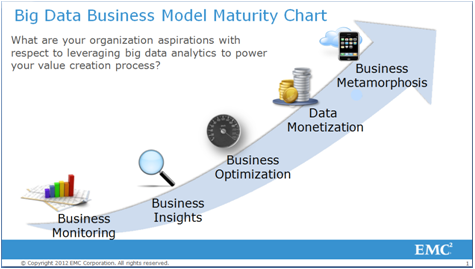
All business applications offer some form of reporting – if you’ve ever seen an information maturity chart, it is the first stage of maturity (see below thanks to an EMC2 slide deck).

Riddle me this then, if the source application (OLTP) provides reporting why do we need a data warehouse? Show reports at a particular point in time? Maybe – (although a lot of users struggle with this and tend to think in current terms). There are a lot of tools that provide adhoc query (OLAP) capabilities so performance the performance of analysis isn’t a real consideration (after all, they could just use an OLAP engine over the OLTP right?).

I think one of the primary reasons is integration. We want to either integrate data from different systems (creating an enterprise view) or we want to supplement current data with with other, richer information (which is really just integration anyway isn’t it). We could even say that business rules and derived information falls into this category.

Here also temporal tables do not negate the need for the data warehouse. The data warehouse is responsible for delivering a consistent, conformed, business verified data that incorporates information from various sources. Nothing changed there (and still the need for a data warehouse).

Finally, lets consider the dimension. That subject orientated view of an object. Its the Product table that tells me everything I need to know about a Product – its category, groupings, margin positions and alike. The dimension is notorious for redundancy and de-normalisation but that’s the price we are prepared to pay for
delivering a single concise view to a user because it breaks down the complexity of the model for the user (they don’t have to combine products to product categories in a query). The idea that we have de-normalise breaks the basic OLTP conventions which force normalisation (after all, we expect 3^rd normal form).

The data warehouse is designed to do this work for us and present the view to the user. Essentially, its just another integration problem but one that’s handled (and hidden) by the data warehouse. Our BI tools (again with the presentation layers) may be able to create these consolidations for us however we are still presented with the issue of uniqueness in related table records (that is, we have to identify which category related to a product at a point in time and the BI tools will not do that for us).

So, are temporal tools a replacement for a data warehouse? I think not, sure they may be able to assist with record change tracking (we haven’t discussed the shift in OLTP resource management). Temporary tables are only a tool and I’d be very careful of anyone that claims they could replace a data warehouse.

MySql Import Issues with Tabular and OldGuids

In my last post, I looked at a MySql connection property that causes loads to fail in Power BI and how you can work around that issue (see here).  In this post, I’ll look at those implications in SSAS Tabular.  In this example, I’ve downloaded the MySql ODBC drivers (both x32 and x64) from here and created ODBC connections (x32 and x64 with the same name) to my MySQL database.

Data is initially imported through the Table Wizard where I have to choose the relational source Others ( OLEDB/ODBC).  This brings me to the Table Import Wizard window (below) where I can choose my ODBC Connection.  Testing the connection proves successful.  So you navigate next a few times until you can chose to import from a list of tables or write a query.

If you choose to select tables (and any) of the tables have Guids in them, the entire load will fail and you are presented with the following errors. 

Here the error is raised by the SQL generated because it is not compliant with MySQL (that is the SQL generated is “Select [calls].* from [calls]” and MySql does not like square brackets).

Far enough, so you continue.  Now that the connection has been created in the model all you need to do to import data is Open the existing connection (existing connections in the model can be viewed by clicking the Connections button in the ribbon () or by selecting “Existing Connections..” from the Model Menu group).  You can then open that connection (either Double Click it or highlight it and press the Open button) and you are presented with the select from tables or write a query).  This time you specify the query (Select * From Calls).  The query validates however, a new error is presented when you try to load data.  Although not specified, it does relate to the OldGuids property.

Now we have to manually edit the connection to specify its properties.  When we do so, we are presented with the following window.  Now I want to build the connection string so specify connection string and select the build option.  Then I can choose the machine data source (btw I set up my ODBC connections as machine sources).

Now I am taken to the drivers creation window (as below).  I don’t need to change anything here (since the connection works anyway), so I will accept the defaults and hit OK.  (Note that the OldGuids property is not an option in the details section of the drivers configuration)

My Connection String has now been specified (note the additional properties in the window and snippet below) and I can add other properties as I need.

Before:

DSN=dsnname;SERVER=server;UID=username;PWD=password;DATABASE=databasename;PORT=3306

After:

DSN=dsnname;SERVER=server;UID=username;PWD=password;DATABASE=databasename;PORT=3306;OldGuids=true;

Then I simply specify my impersonation and I am right to go (noting that I must write a query).