Life is ironic: After the short rant about company willingness to use data mining, I was asked to mentor a client on it! They wanted to investigate the predictive capability of time series modelling.
Regardless of whether mining is applied in a descriptive or predictive manner, Analysis Services makes it easy to include some facet of data mining into operations (or at least investigate it). The use of DMX (Data Mining Extensions) makes it simple to create the model and obtain values from it and is equivalent to SQL for data mining. Some are surprised to find that BIDS is not required to create, train and query the model.
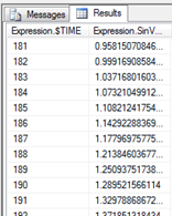
In this example, we will predict a sinusoidal curve using the time series algorithm. The curve takes the form as seen in the picture below;

There are three basic steps to obtaining the predictions. Firstly, the model has to be created. For all intensive purposes, this is the implementation of one mining algorithm with a distinct set of parameters. The model relies on a structure which defines the meta-data for input but, just as in BIDS, the creation of a model will automatically create the structure for model use. Secondly, the model needs to be trained, and finally, the model can be queried.
Model Creation
A model can be created by simply using the CREATE MIING MODEL SYNATX (as below). Model columns must be defined by name, data type and content type. Content types define behaviour (eg role as key and time) and data behaviour (DISCRETE, CONTINUOUS, DISCRETIZED). Additionally, prediction columns (ones being predicted) require a prediction request (PREDICT OR PREDICT_ONLY).
CREATE MINING MODEL [SinPredict]
(
Degree LONG KEY TIME
, SinValue DOUBLE CONTINUOUS PREDICT
) USING
MICROSOFT_TIME_SERIES
WITH DRILLTHROUGH
As stated, the creation of the model will automatically create a structure. By default, the structure name will be the models name with a ‘_Structure’ suffix (eg SinPredict_Structure). Had we wished to specify the structure first (also perfectly valid) and append the model to it, we could use the create / alter-append syntax below.
— Create structure
CREATE MINING STRUCTURE [SinTimeSeries]
(
Degree LONG KEY TIME
, SinValue DOUBLE CONTINUOUS
)
— Append the model
ALTER MINING STRUCTURE [SinTimeSeries]
ADD MINING MODEL [SinPredict]
(
Degree
, SinValue PREDICT
) USING MICROSOFT_TIME_SERIES
WITH DRILLTHROUGH
Model Training
Once the model has been created, it can be trained (or populated). Queries run against an unprocessed model will err as will trying to re-train the model without first deleting prior contents. The generic form of training is an insert statement. For example,
INSERT INTO Model(Columns)
<< The RowSet >>
Since the generation of sinusoidal data for training can be easily accomplished with a CTE, an OPENROWSET statement to an SQL server can be used to populate the model (note the cte provided the chart above). The DMX query to populate the model is;
INSERT INTO SinPredict(Degree, SinValue)
OPENROWSET(‘SQLOLEDB.1’
, ‘Provider=SQLOLEDB.1;Integrated Security=SSPI;Initial Catalog=master;Data Source=.\SQL2008R2’
, ‘ WITH Deg AS
(
SELECT CAST(1 AS MONEY) AS Deg
UNION ALL SELECT Deg + 1
FROM Deg
WHERE Deg < 180
)
SELECT *, CAST(SIN(Deg/9) AS MONEY) AS SinValue
FROM Deg OPTION (MAXRECURSION 180)’
)
Note that, by default, rowset queries are not enabled in SSAS and shouls be configured in server properties. These are basic (open rowset queries) and advanced properties (allowed providers).

Model Prediction
Once the model has been trained, it can be queried. For time series, we can use the PREDICT or PREDICTTIMESERIES
functions (both achieve the same result) and forecasts the next n values. By default, the model returns results in the nested form which can be flattened using the keyword (as below).
SELECT PREDICTTIMESERIES(SinValue, 20)
FROM [SinPredict]
 |
 |
SELECT FLATTENED PREDICTTIMESERIES(SinValue, 20)
FROM [SinPredict]
One of the interesting observations about time series predictions is that the sequence identifier values are incremented from the last value in the training record set. These values are not predicted as part of the prediction function which becomes apparent when using smart keys. For example a date smart key in the form of YYYYMMDD with the last training value of 20110520 (20-May-2011) will predict incrementally from 21-May. When 30 is reached, the next sequence number is 31, then 32 and so on.
Conclusion
The use of DMX offers a simple way of implementing SSAS data mining. This simple example demonstrates how to create a time series model, train it and then predict from it.
