Creating Tables in Excel with VBA and External Data – Part II

In Part I, we looked at adding a data table to a Workbook which uses an external data source (we used OLAP but the process can be applied to any source). This post looks at manipulating an existing table.

Without VBA, we can manually manage the table – both the its properties and the underlying query. Simply right click on the table and select the Edit Query.. or External Data Properties from the popup menu. Changes are made to the table data are made automatically.

If we chose to edit the query, we can simply overwrite the Command Text (as seen in the image below). These changes well be automatically applied (including resizing the table by rows or columns for a different sized data set) once the OK button is clicked.

For External Data Properties, we can configure how the table reacts with new data. For example, you may notice that, the table accommodates additional rows and columns however, when the query returns a table with fewer rows and columns, the table retains its old sizing (number of columns) and includes a blank columns (for data that previously existed). You can manually resize this (dragging the bounds of the tables border) or set the properties of the table to overwrite existing data. If you want to ensure that this option exists and that new sizes are automatically incorporated into the table – make sure that the check box for Overwrite is marked in External Data Properties.

VBA

Now to the VBA – As commandant Lassard would say “There are many, many, many, many fine reasons to use VBA”. We have so much flexibility but let’s keep it simple, here’s what we I’ve set up.

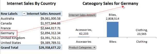
Cell B1 is data validated based on the cell range D1:D2 – nice and simple. When we change that cell, the table updates for the new country.

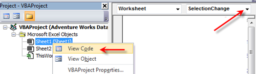
In order to determine if the there is a change in or data (the Country selected) we have to create a worksheet event to capture and test the change. I have gone into this in some detail here and the code is below. Note that this needs to be added to the sheet code (not in a separate bas module). All we do is check that our only B1 is updated and then call the refresh subroutine.

Private Sub Worksheet_Change(ByVal Target As Range)

  ‘ update table if cell 1,B is changed
If Target.Cells.Count = 1 And Target.Cells.Row = 1 And Target.Cells.Column = 2 Then UpdateMyTable

End Sub

Now for the updating component – the bit that’s called when cell(B1) is changed. I think this is pretty straight forward but I’ll walk through it anyway. First, the code;

Public Sub UpdateMyTable()

  ‘ ensure that any new changes are reflected in the table dimensions
Sheet1.ListObjects(“Table_abax_sql3”).QueryTable.RefreshStyle = xlOverwriteCells

  ‘ set the comand text
Sheet1.ListObjects(“Table_abax_sql3”).QueryTable.CommandText = NewQuery(Sheet1.Cells(1, 2))
Sheet1.ListObjects(“Table_abax_sql3”).Refresh

End Sub

Private Function NewQuery(Country As String) As String

NewQuery = “select {[Measures].[Reseller Sales Amount] } on 0, ” & _
“[Product].[Category].[Category] on 1 ” & _
“from [Adventure Works] ” & _
“where [Geography].[Geography].[Country].&[” & Country & “]”

End Function

I’ve kept the same format as in the original post. The function NewQuery determines what the MDX should be – based on the provided country. All we is set the tables command to the new mdx (in (QueryTable.CommandText)) and refresh it.

I’ve also set the refresh style so that any changes in the command (grid size) are automatically reflected in the worksheet table.

That’s about the size of it! – I hope you find it useful.

Creating Tables in Excel with VBA and External Data – Part I

This post looks at how we can add a table to an Excel sheet which uses a MDX query as its source. This is a very handy feature to use for a couple reasons;

1. The table retains the connection OLAP source (hence can be updated by a user at will)
2. We can use it to extract data from MOLAP or tabular sources (i.e. run MDX or DAX)
3. We can define complex queries to return a result set that cannot be obtained with a pivot table

Note that most workarounds for creating a table from OLAP sources rely on the creation of the pivot table, its formatting is a tabular source and a copy and paste the values. Hardly an attractive option!

1. We can use the table!! – (This is really important for certain activities like data mining table analysis)

How to Do It

We’ll look at a simple query from adventure works;

select [Measures].[Reseller Sales Amount] on 0,
[Product].[Category].[Category] on 1
from [Adventure Works]
where [Geography].[Geography].[Country].&[Australia]

and an OLEDB connection string (note the OLEDB specification at the start of the string)

OLEDB;Provider=MSOLAP;Data Source=@server;Initial Catalog=Adventure Works DW 2008R2;

I have incorporated those to strings into 2 functions (MyQuery and MyConnectionString) – this just removes some of the clutter from the code.

Now we just need to use the ListObjects.Add method. The code (now in with all Sub’s and Functions) is pretty much the bare bones you need to add the table. In other posts, I’ll look into higher level of control for the output.

The CODE

The complete code is shown below. Ive included everything so it can simply be pasted into a new VB module

Sub CreateTable()

  With Sheet1.ListObjects.Add(SourceType:=0 _
, Source:=MyConnectionString() _
, Destination:=Range(“$A$1”) _
                            ).QueryTable
.CommandType = xlCmdDefault
.CommandText = MyQuery()
.ListObject.DisplayName = “MyMDXQueryTable”
.Refresh BackgroundQuery:=False
.PreserveColumnInfo = False

  End With

End Sub

Private Function MyQuery() As String

     MyQuery = “select [Measures].[Reseller Sales Amount] on 0, ” & _
“[Product].[Category].[Category] on 1 ” & _
“from [Adventure Works] ” & _
“where [Geography].[Geography].[Country].&[Australia]”

End Function

Private Function MyConnectionString() As String

     MyConnectionString = “OLEDB;Provider=MSOLAP;Data Source=@server;Initial Catalog=Adventure Works DW 2008R2;”

End Function

Walk through

This is pretty much the bare bones approach. As code walk through (see Sub CreateTable), we add the list object specifying its connection string and destination, set the command and refresh info. The only statement that is not entirely necessary is naming the table (see .ListObject.DisplayName) but I tend to think is a good idea because we will want to refer to it by name at a later stage.

Out Come

The code will add a table like the one in the following image. The field names are fully qualified which is not that nice and we will look at how this can be changed in another post. For now, our purpose is to get a table is in the workbook (the purpose of this post) so that it can be used as a table and refreshed.

PS – the code above adds the listobject by reference to the sheet within VBA (see Sheet1.ListObjects). Its probably worthwhile to point out that this is the sheet reference (ie the number of the sheet in the book) and not the name of the sheet.

One more thing – when the query uses refers to a attributes in a hierarchy the OLEDB result set (table) will include parent attributes of the hierarchy as a column. This is nothing to worry about for the moment!

Next – changing the tables query.

Pivot Filtering with Cell Selection and VBA

This post looks at applying data filters in Excel workbooks with sheet ‘click’ functionality for filtering. The purpose of this is to provide a rich user experience for reporting within Excel. With these types of reports, you present some data in a pivot which is used to as a source filter for other parts of your report (or worksheet). Consider the situation below; when you click on one of the country names in the pivot, the chart is automatically updated to filter for that country. Clicking on any other area of the pivot removes any chart filter.

Why would you do this?

Monthly reporting workbooks are often treated as report packs and designed in lieu of an enterprise reporting system. Even where such an enterprise reporting system are in-place, the reporting environments are usually not flexible enough to provide the business what they need for monthly reporting and so the workbooks are bundled together in Excel. These workbooks can be extended to have highly interactive functionality that mimics high-end reporting tools.

While you could achieve these results with a slicer, the automation of the action may provide a nicer experience for the user because it removes the slicer clutter from the page and allows a direct association with the data being investigated.

How to Do IT

Achieving this functionality is conceptually pretty simple (and soon programmatically simple too J), all we need to do is;

1. Listen for changes in the cell position on a worksheet.
2. When a change is detected, we check that the change was to our source pivot
3. Determine the filter value (ie what value was clicked in the pivot) … and
4. Apply that value to the slicer for the chart.

These items are now discussed individually.

Work Book Setup

In this example, I am using an Adventure Works connection with a pivot table and pivot chart. The pivot table (the one you click a cell on) is called ‘country_sales’. This uses the customer.country hierarchy from adventure works. The pivot chart has a slicer linked to it (and the name of the slicer is ‘Slicer_Counrty’). Note that the same hierarchy must be used for both the slicer and pivot table.

Listening for changes in the worksheet

Each worksheet has its own code module with defined events. An event is a subroutine that is ‘inbuilt’ into Excel and fired when something happens in Excel (for example, when the user changes the active cell). You can see the worksheets module by double clicking the sheet in the project explorer or with a right-click and ‘View Code’ and see the events by selecting them from the dropdown (as shown below).

When you do this (and choose the event SelectionChange), you’ll see the following subroutine added to your module

Private Sub Worksheet_SelectionChange(ByVal Target As Range)
End Sub

Now, that this has been added, this procedure will fire every time you change selection cells on Sheet1. It also may be worthwhile to note that the Target parameter refers to the range of cells that’s selected (as part of the selection). Because you can select more than 1 cell, we want to check for single cell selection so we simply exit the sub if there is more than on cell in the range.

If (Target.Cells.Count <> 1) Then Exit Sub

Detecting the Source Pivot and the Active Cell Value

There are some pretty handy functions to determine if the active cell relates to a pivot table, and if it does, that the member name is and what its value is. These relate to the activecell and are the properties

.PivotTable

.PivotItem

.PivotField

Thus, in order to determine what the name of a pivot table for the active cell we would simply write;

Dim source_pivot_name As String
source_pivot_name = ActiveCell.PivotTable.Name

The name (MDX value) of a column could be determined by ActiveCell.PivotItem.Name

and the (MDX) name of the attribute
(Dimension.Hierarchy.Level) determined by  ActiveCell.PivotField.Name

For example, if I click on the France ‘country columns’ in my pivot table, I would get the following values.

ActiveCell.PivotTable.Name	“country_sales”
ActiveCell.PivotField.Name	“[Customer].[Country].[Country]”
ActiveCell.PivotItem.Name	“[Customer].[Country].&[France]”

Note that the pivot values references are to the object model (ie the Pivot object). If the cell your referring to (the activecell) is not part of a pivot table, you’ll get an error. This is pretty easy to catch with some error trapping (see final code).

Assuming that the user clicked on a cell in the pivot (I will leave the checks for the final code) we have all the values that we need and can then set the slicer.

Applying the filter to the Slicer

I have discussed applying how to apply slicer value in VBA in this post. For brevity, I’ll just include the essential items. We simply make a reference to the slicer (SlicerCache) and set its value.

Dim sC As SlicerCache
Set sC = ActiveWorkbook.SlicerCaches(“Slicer_Country”)
sC.VisibleSlicerItemsList = Array(ActiveCell.PivotItem.Name)

If I want to remove the slicers current filter (when no ‘country is needed), I can do that with this code;

sC.ClearManualFilter

Complete Code

The following code demonstrates the complete solution. I have included updating the ‘title’ of the chart and error traps to determine if a ‘non country’ part of the pivot was chosen.

Private Sub Worksheet_SelectionChange(ByVal Target As Range)
  If (Target.Cells.Count <> 1) Then Exit Sub
  Dim source_pivot_name As String
  source_pivot_name = “”
  Dim source_field As String
  source_field = “”
  Dim source_attribute As String
  source_attribute = “”
  Dim sC As SlicerCache
  Set sC = ActiveWorkbook.SlicerCaches(“Slicer_Country”)
  On Error GoTo continue
  ‘try and get the active cells pivot table name
source_pivot_name = ActiveCell.PivotTable.Name
continue:
‘we can only apply a filter if we are on our ‘selection pivot’
If source_pivot_name = “country_sales” Then
  ‘note the name must go first so we can check for a ‘Row Labels’ Position
On Error GoTo continue2
source_attribute = ActiveCell.PivotField.Name
On Error GoTo continue3
source_field = ActiveCell.PivotItem.Name
continue2:
continue3:
‘check we have the correct source
If (Len(source_attribute) > 10 And Left(source_attribute, 10) = “[Measures]”) Or _
(source_field = “” And source_attribute = “[Customer].[Country].[Country]”) Then
‘set to all
sC.ClearManualFilter
Sheet1.Cells(11, 4) = “Category Sales for All Areas”
Else
sC.VisibleSlicerItemsList = Array(source_field)
Sheet1.Cells(11, 4) = “Category Sales for ” & ActiveCell.Value
End If
 End If
End Sub

Conclusion

Adding some interactive functionality to a pivot is a pretty simple exercise which relates to the identification of a cell value and, in turn setting a slicer. This improves the end user experience for excel reporting books.

Viva Excel and black IT J. A little cheeky!

Accessing the Slicer through VBA

There may be times when we want to programmatically control slicers through VBA. For example, we may want to default a date to the current date or set a cost centre depending on who has opened the book. This post looks how a slicer can be controlled through VBA.

In this example, we have added a slicer to a worksheet that uses a date hierarchy as its source. Because, we have included all levels of the hierarchy when the slicer was setup, we get three individual slicers for each level of the hierarchy.

If we look at the settings for the slicer (right click on the slicer and select slicer settings), we can see that the slicer has a name and each level of the slicer hierarchy maintains the hierarchy level name. For example, the Slicer_Dates_Hie below has a level Year, Month and Day. Although we can change the name (for example the name Year in the picture below), the slicer retains the mdx level that the slicer belongs to.

Accessing the Slicer

We can access the slicer through the SlicerCaches object. This is as simple as declaring the slicer cache and referencing it to the name of the slicer we want to use. For example;

Dim sC As SlicerCache
Set sC = ActiveWorkbook.SlicerCaches(“Slicer_Dates_Hie”)

Navigating the Structure of the Slicer

Once we have a reference to the slicer we can navigate its structure using SlicerCacheLevels. For example we can determine the number of levels of the slicer and iterate over them with the following code.

Dim sC As SlicerCache
Dim sL As SlicerCacheLevel
Set sC = ActiveWorkbook.SlicerCaches(“Slicer_Dates_Hie”)

For Each sL In sC.SlicerCacheLevels
Debug.Print “Level ” + CStr(sL.Ordinal) + ” –> ” + sL.Name
Next sL

Naturally, the level can be accessed through the cache level ordinal to produce the same result. The highest level (year) takes the value 1 which increments for each level from the first level. There is always a level (ie level 1) even if the slicer is based on a single attribute.

Set sC = ActiveWorkbook.SlicerCaches(“Slicer_Dates_Hie”)
For i = 1 To sC.SlicerCacheLevels.Count
Debug.Print “Level ” + CStr(i) + ” –> ” + sC.SlicerCacheLevels(i).Name
Next i

Slicer Data Members

We can gain access to the data items through slicer items, as mdx attributes, they have a caption, value and a key (member unique name). For example the year 2011 in this slicer has a value of 2011 and a name (MDX unique name) of [Dates].[Dates Hie].[Year].&[2011]

Dim sC As SlicerCache
Dim SL As SlicerCacheLevel
Dim sI As SlicerItem

Set sC = ActiveWorkbook.SlicerCaches(“Slicer_Dates_Hie”)
Set SL = sC.SlicerCacheLevels(1)
Debug.Print “——————————————————————————”

For Each sI In SL.SlicerItems
Debug.Print “Caption –> ” & sI.Caption
Debug.Print “Value –> ” + CStr(sI.Value)
Debug.Print “Unique Name –> ” + sI.Name
Debug.Print “——————————————————————————”

Next

Setting the Slicer Value

Slicer item selection must be set through the visible slicer items list and is specified using an array. For example, we could set the SlicerCache (selected items) to 2011 and 2012 with the following code;

sC.VisibleSlicerItemsList = Array(“[Dates].[Dates Hie].[Year].&[2011]”, “[Dates].[Dates Hie].[Year].&[2012]”)

The name selected must be a data member of the level. If not a runtime error will occur (as below)

Once the values are set, connected pivots are updated immediately

Member Iteration

Members can be easily iterated using the following code;

Dim sC As SlicerCache 
Dim SL As SlicerCacheLevel 
Dim sI As SlicerItem
Set sC = ActiveWorkbook.SlicerCaches("Slicer_Dates_Hie") 
Set SL = sC.SlicerCacheLevels(2)
For Each sI In SL.SlicerItems    
 sC.VisibleSlicerItemsList = Array(sI.Name) 
Next

Conclusion

The control of slicers through VBA could be used to provide some very nice personalisation to work books.

NB:  If you liked this post you might be interested in this one.  In it, I discuss setting slicers through cell association to pivot rows.