Pivot Filtering with Cell Selection and VBA

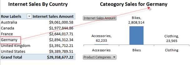
This post looks at applying data filters in Excel workbooks with sheet ‘click’ functionality for filtering. The purpose of this is to provide a rich user experience for reporting within Excel. With these types of reports, you present some data in a pivot which is used to as a source filter for other parts of your report (or worksheet). Consider the situation below; when you click on one of the country names in the pivot, the chart is automatically updated to filter for that country. Clicking on any other area of the pivot removes any chart filter.

Why would you do this?

Monthly reporting workbooks are often treated as report packs and designed in lieu of an enterprise reporting system. Even where such an enterprise reporting system are in-place, the reporting environments are usually not flexible enough to provide the business what they need for monthly reporting and so the workbooks are bundled together in Excel. These workbooks can be extended to have highly interactive functionality that mimics high-end reporting tools.

While you could achieve these results with a slicer, the automation of the action may provide a nicer experience for the user because it removes the slicer clutter from the page and allows a direct association with the data being investigated.

How to Do IT

Achieving this functionality is conceptually pretty simple (and soon programmatically simple too J), all we need to do is;

1. Listen for changes in the cell position on a worksheet.
2. When a change is detected, we check that the change was to our source pivot
3. Determine the filter value (ie what value was clicked in the pivot) … and
4. Apply that value to the slicer for the chart.

These items are now discussed individually.

Work Book Setup

In this example, I am using an Adventure Works connection with a pivot table and pivot chart. The pivot table (the one you click a cell on) is called ‘country_sales’. This uses the customer.country hierarchy from adventure works. The pivot chart has a slicer linked to it (and the name of the slicer is ‘Slicer_Counrty’). Note that the same hierarchy must be used for both the slicer and pivot table.

Listening for changes in the worksheet

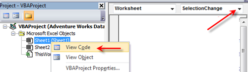
Each worksheet has its own code module with defined events. An event is a subroutine that is ‘inbuilt’ into Excel and fired when something happens in Excel (for example, when the user changes the active cell). You can see the worksheets module by double clicking the sheet in the project explorer or with a right-click and ‘View Code’ and see the events by selecting them from the dropdown (as shown below).

When you do this (and choose the event SelectionChange), you’ll see the following subroutine added to your module

Private Sub Worksheet_SelectionChange(ByVal Target As Range)
End Sub

Now, that this has been added, this procedure will fire every time you change selection cells on Sheet1. It also may be worthwhile to note that the Target parameter refers to the range of cells that’s selected (as part of the selection). Because you can select more than 1 cell, we want to check for single cell selection so we simply exit the sub if there is more than on cell in the range.

If (Target.Cells.Count <> 1) Then Exit Sub

Detecting the Source Pivot and the Active Cell Value

There are some pretty handy functions to determine if the active cell relates to a pivot table, and if it does, that the member name is and what its value is. These relate to the activecell and are the properties

.PivotTable

.PivotItem

.PivotField

Thus, in order to determine what the name of a pivot table for the active cell we would simply write;

Dim source_pivot_name As String
source_pivot_name = ActiveCell.PivotTable.Name

The name (MDX value) of a column could be determined by ActiveCell.PivotItem.Name

and the (MDX) name of the attribute
(Dimension.Hierarchy.Level) determined by  ActiveCell.PivotField.Name

For example, if I click on the France ‘country columns’ in my pivot table, I would get the following values.

ActiveCell.PivotTable.Name	“country_sales”
ActiveCell.PivotField.Name	“[Customer].[Country].[Country]”
ActiveCell.PivotItem.Name	“[Customer].[Country].&[France]”

Note that the pivot values references are to the object model (ie the Pivot object). If the cell your referring to (the activecell) is not part of a pivot table, you’ll get an error. This is pretty easy to catch with some error trapping (see final code).

Assuming that the user clicked on a cell in the pivot (I will leave the checks for the final code) we have all the values that we need and can then set the slicer.

Applying the filter to the Slicer

I have discussed applying how to apply slicer value in VBA in this post. For brevity, I’ll just include the essential items. We simply make a reference to the slicer (SlicerCache) and set its value.

Dim sC As SlicerCache
Set sC = ActiveWorkbook.SlicerCaches(“Slicer_Country”)
sC.VisibleSlicerItemsList = Array(ActiveCell.PivotItem.Name)

If I want to remove the slicers current filter (when no ‘country is needed), I can do that with this code;

sC.ClearManualFilter

Complete Code

The following code demonstrates the complete solution. I have included updating the ‘title’ of the chart and error traps to determine if a ‘non country’ part of the pivot was chosen.

Private Sub Worksheet_SelectionChange(ByVal Target As Range)
  If (Target.Cells.Count <> 1) Then Exit Sub
  Dim source_pivot_name As String
  source_pivot_name = “”
  Dim source_field As String
  source_field = “”
  Dim source_attribute As String
  source_attribute = “”
  Dim sC As SlicerCache
  Set sC = ActiveWorkbook.SlicerCaches(“Slicer_Country”)
  On Error GoTo continue
  ‘try and get the active cells pivot table name
source_pivot_name = ActiveCell.PivotTable.Name
continue:
‘we can only apply a filter if we are on our ‘selection pivot’
If source_pivot_name = “country_sales” Then
  ‘note the name must go first so we can check for a ‘Row Labels’ Position
On Error GoTo continue2
source_attribute = ActiveCell.PivotField.Name
On Error GoTo continue3
source_field = ActiveCell.PivotItem.Name
continue2:
continue3:
‘check we have the correct source
If (Len(source_attribute) > 10 And Left(source_attribute, 10) = “[Measures]”) Or _
(source_field = “” And source_attribute = “[Customer].[Country].[Country]”) Then
‘set to all
sC.ClearManualFilter
Sheet1.Cells(11, 4) = “Category Sales for All Areas”
Else
sC.VisibleSlicerItemsList = Array(source_field)
Sheet1.Cells(11, 4) = “Category Sales for ” & ActiveCell.Value
End If
 End If
End Sub

Conclusion

Adding some interactive functionality to a pivot is a pretty simple exercise which relates to the identification of a cell value and, in turn setting a slicer. This improves the end user experience for excel reporting books.

Viva Excel and black IT J. A little cheeky!